|
||||||||
|
||||||||

|

Implementing OLAP in Delphi Applications
Natalia Elmanova More details on using ADO
Extensions in OLAP Basics
What are OLAP and Data Warehousing? Client-side OLAP Applications in
Brief
How to Implement a Client-side OLAP Using MS SQL Server 7.0 OLAP
services and Delphi ADO components
OLAP Services Architecture Using ADO MD Extensions
ADO MD Objects ADOMD Usage Examples
Using the Catalog Object and its
Collections Pros and Cons of Delphi server-side
OLAP applications
Conclusion
In this article, we will
talk about using ADO for On-Line Analytical Processing (OLAP) - the data
management techniques that are widely used in decision support systems and data
warehousing. We will also discuss two ways of implementing OLAP with ADO and
Delphi, such as using client-side OLAP and server-side one. OLAP
Basics
Enterprise information
systems contain, as a rule, different user applications. Among them, there are
applications for decision support, multidimensional data analysis, obtaining
trends, receiving statistics, and several other tasks. They usually have an advanced
user interface that includes business graphics and provides functionality for
obtaining various aggregate data - sums, counts, averages, maximal and minimal
values, and so on. Behind the user interface
of such decision support applications, there is an implementation of providing
such analysis. Such implementation is based on OLAP - this term, that
may be new to the most of our readers, is explained in the next section. What
are OLAP and Data Warehousing?
OLAP - On-Line
Analytical Processing
is a popular technology for multidimensional business analysis. It is based on
the multidimensional data model that will be discussed later. The concept of
OLAP was described in 1993 by Dr. E.F.Codd, the well-known database researcher
and inventor of the relational database model. At present time, OLAP support is
implemented in different databases and tools. For example, the most of the
database servers provide OLAP facilities, sometimes as separate specializes
data storages and tools for operating them (e.g. ORACLE Express OLAP,
Microsoft SQL Server 7.0 OLAP Services, and so on). OLAP is a key component in data
warehousing. Data warehousing is the process of collecting and
sifting data from different information systems and making the resulting
information available to end users for analysis and reporting. Data warehouse
can be used to describe these stores of collected and summarized information
that is available for browsing by users. In most cases, there is no
easy way to find the information necessary for making a decision in relational
databases. For example, the data structures can be difficult for the end user
to understand, or the user questions are quite complex when being expressed in
SQL language. Imagine the following
example. To get an answer to the question like "Who are the top customers
in each region for the year 1998 arranged by quarter?", we must execute a
lot of particular queries to obtain a two-dimensional subset of aggregate
values and then show this subset to the user. That is why any OLAP
implementation contains advanced query tools, which hide the database
complexity from the end user. Talking about OLAP tools,
we should say, that OLAP facilities are also can be found in development tools
and office applications. Contrary to the server-side OLAP, such as ORACLE
Express OLAP or Microsoft SQL Server 7.0 OLAP Services, these facilities
usually implement client-side OLAP. For example, within Microsoft Excel 2000, a
new PivotTable dynamic view function will provide connectivity between Excel spreadsheets
and OLE DB Provider for SQL Server OLAP Services. This gives us an
ability to create a local subset from a larger aggregate data from database
server. As for Delphi, its
Enterprise version comes with a set of client-side OLAP components, which can
be found in the Decision Cube page of the Component Palette. Later, we
will say several words about them. Using OLE DB Provider
for SQL Server OLAP Services, Delphi applications can also connect to
server-side OLAP storages to retrieve aggregate data to end users. Later we
will see how to create such applications. Before we create decision
support applications, let's spend some time discussing what multidimensional
cubes are, and what data they contain. What
Are Decision Cubes?
In this section, we will
discuss the Decision Cube and OLAP concepts in details. To provide a simple
example of what multidimensional analysis is, we will use the NorthWind
database on the Microsoft SQL Server and we will create a view based on several
tables from it. Here is the SQL source for this view.
This view returns us a
dataset with nearly complete information on the all orders that will be used in
the examples in this article. If we use Microsoft Access,
the same view may look like the one shown below.
The resulting recordset for
CustomerID, OrderDate, CompanyName, Freight, ShipCountry, and Payment
fields is shown in the table below.
What are the aggregate data
that can be obtained from such table or view? Usually they can answer to
the following typical questions:
There may be different
questions, depending of the kind of the company business, but we have listed
just typical ones. Since we are working with
the data that resides in a database, we need to translate these human-readable
questions into SQL queries. For example:
Note. In some cases, such text queries
can be translated to its SQL equivalent with the help of Microsoft English
Query. As we may expect, the
result returned by execution of any of the queries shown above will return some
number. As you can see from the SQL query source, we can replace 'France'
to 'Austria', or any other country name, execute this query again,
and obtain another value. Doing this with all customer names, we will obtain a
set of values that can be presented in a simple table shown below.
The table shown above
contains aggregate data and can be considered as one-dimensional set of values.
Now let's look at the
second and the third query that contain two conditions in the WHERE
clause.
If we run this query
changing the Country value or the CompanyName value for every
country or company name we have in the database, we will get a 2-dimensional
set of values shown in the following table. CompanyName
This set of values is
called cross table or pivot table. Creating such tables from the
original data is the simple data processing function found in many spreadsheet
packages like Microsoft Excel. Now let's look at the
fourth query.
This query contains three
conditions in the WHERE clause. Therefore, if we want to get all
possible results for this query, we must supply different data for all three
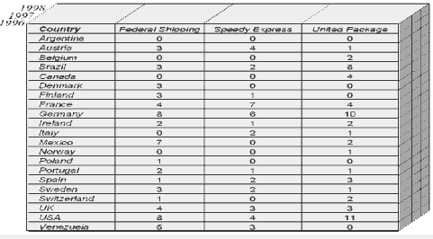
parameters. As a result, we will get a 3-dimensional set of values that can be
presented as a cube shown in the figure below.
Any cell of this cube
contains a numeric value that results from a query similar to query shown
above, but with different parameter values in the WHERE clause. If we slice the cube by a
plane parallel to one of the cube edge, we can get different types of the
two-dimensional tables. Such tables are called cross-sections (or slices)
of such cube. The example of such slices is shown below. Orders in the USA
Orders delivered by Federal Shipping
If we create a sample query
with 4 or more conditions in the WHERE clause, we will get a
4-dimensional (or 5-dimensional, 6-dimensional, etc.) set of values. It should be clear, that
along with sums and counts, we can also put into the cube cells maximal,
minimal, and average values, i.e. aggregate SQL functions such as MIN, MAX,
AVG. Sometimes these aggregate values are called summaries, and
variables used in queries are called dimensions. The original source
data that is summarized (e.g. payments) is called measures. Within each dimension of
the cube, data can be organized into a hierarchy that represents detail levels
of the data. For instance, within the OrderDate dimension, there can be
the following levels: years, quarters, months, and days. This multidimensional data
model makes it simple for users to formulate complex queries, arrange data in a
report, switch from summary to detailed data, and filter or slice data to
create different subsets. As we have mentioned
earlier, such multidimensional analysis can be provided both on a database
server and inside a client application. We will begin with a short discussion
of the possible ways of implementing client-side OLAP. Client-side
OLAP Applications in Brief
In this section, we will
discuss in brief possible ways of creating Delphi client-side OLAP
applications. How to
Implement a Client-side OLAP
As we have said before,
Delphi Enterprise includes a set of Decision Cube components for
implementing client-side OLAP. These components provide a convenient user
interface of analytical applications. But using them with ADO data sources will
face several difficulties. First, the Decision Cube
components do not support TWideStringField fields. So, we need to obtain
the resulting dataset without such fields (such as we have done in the view
created earlier). However, this way of solving the problem of unsupported
WideString data in Decision Cube components is not universal. For example, we
may have not enough privileges to create database views. In this case, we need
to create calculated fields that contain non-unicode versions of the WideString
fields and use them to create cube dimensions, or redefine all WideString
fields as TString fields by replacing all "WideString"
substrings to "String" substrings in the appropriate *.pas
and *.dfm files. Second, the TDecisionQuery
component that contains a specialized form of TQuery used to define the
data in a decision cube is a fully BDE-oriented component. In Delphi 5, it does
not work with ADO data sources at all. We can, of course, replace
the TDecisionQuery component with any ADO dataset component (e.g., TADOQuery),
and type the query for the calculating summaries manually, for example:
In this case, we can create
an application with a convenient user interface, containing grids, charts and
controls to hide, show, expand and collapse dimensions, and, at design time, it
will look beautiful. However, and it is the third problem, when we run such
application, its run-time behavior becomes strange: not all of the data is
presented correctly (for example, some data is lost), indexes for cubes are
calculated significantly more slowly than at design time, the Decision Cube
capacity appears to be low even a dataset is small, and so on. Transferring
data to the client dataset also does not improve the situation. In fact, this
is the most serious reason not to use these components with ADO data sources. However,
we expect that these disadvantages will be improved in the next versions of
Delphi. The radical way of how to
solve these three problems is to edit the source code of the Decision Cube components.
However, after that, you should not expect any support from Borland in the case
of any problems with such components. What should be recommended
for implementing client-side OLAP for ADO data sources instead of using
Decision Cube? First, you can use Excel automation, and, in this case, your
applications could provide all Excel Pivot Table services for your
users. However, in this case, your users must have Excel installed. Second, you
can calculate summaries in your code and use ordinary grids and charts. Pros
and Cons of Client-side OLAP Applications
In this section, we will
try to show you the advantages and disadvantages of using client-side OLAP. Let's
start with the "bright" part of the client-side OLAP. The advantage of
client-side OLAP applications is that in this case, we can provide on-line
analytical processing possibilities for any data source. It does not matter,
whether this data source provides OLAP services itself. It is the most commonly
way to analyze data on desktop databases, SQL servers that do not have its own
OLAP implementations (such as InterBase), data that comes from various ODBC and
OLE DB data sources, and so on. Unfortunately, that is all, what can be said
about advantages of this approach. The disadvantages of
client-side OLAP are very serious, and you must remember about them before
starting to create such applications. First, the client-side OLAP
applications can consume a lot of memory and produce a serious traffic, as they
bring a lot of data from the database server to the client application. Therefore,
the amount of such data should be estimated correctly, and these estimations
must include the possible growth of database in the future. In addition, this
restricts the amount of dimensions. In a general case, for any client-side OLAP
tool, using more than six of them is not recommended. Second, at the time of this
writing, the particular Delphi implementation of client-side OLAP components is
not applicable for using with ADO data sources. We hope this to be improved in
the next version of Delphi. Another way to create OLAP
applications is to use the server-side OLAP. As we will see in the next
section, server-side OLAP is free from the disadvantage like bringing all
summaries to the client, and can be used with large data sources. Now we will discuss the
second way of implementing OLAP. It is to use server-side OLAP extensions
implemented in Microsoft SQL Server 7.0 along with Delphi ADO components or ADO
MD extensions. We will begin with creating
OLAP cubes with the Microsoft SQL Server OLAP Manager. Then we will continue
with creating several applications for querying such cubes using the OpenSchema
method, and querying the cubes using Multidimensional Expressions that are
extensions of the SQL language for querying OLAP cubes. And, at the next
section, we will show how to use ADO MD extensions in Delphi server-side OLAP
applications. Using MS
SQL Server 7.0 OLAP services and Delphi ADO components
In this section, we will
provide one of the ways, how to use ADO MD extensions and create applications,
which use server-side OLAP provided by MS SQL Server 7.0 OLAP services. OLAP
Services Architecture
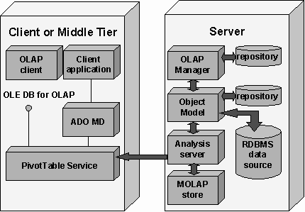
SQL Server 7.0 OLAP
Services consist of server and client components. The client components can
also be used as middle-tier software in multi-tier systems.
On the server side, the
OLAP server operates as a Microsoft Windows NT service and provides the core
computational functionality. OLAP Manager is the built-in administrative user
interface for OLAP Services. It can be executed on a computer separate from the
OLAP server. It allows the database administrator to design OLAP data models,
access information in RDBMS stores, design aggregations, and populate OLAP data
stores. The OLAP metadata definitions are stored in a special repository. It is essential that OLAP
Services can access source data not only in SQL Server, but in any data source,
which can be available through OLE DB data providers. On the client side, OLAP
Services includes a component called PivotTable Service. PivotTable
Service is designed to connect OLAP client applications to the OLAP
Services server. All access to data managed by OLAP Services is provided by
this service through the OLE DB for OLAP interface. Creating
OLAP cubes
Before creating any Delphi
application, we need to create an essential part of a whole server-side OLAP
system. This part is a multidimensional OLAP cube, which is stored and
maintained by a database server. We consider you have
already installed Microsoft SQL Server 7.0. Now, we need to install also SQL
Server 7.0 OLAP Services that are provided with Microsoft SQL Server 7.0 and
can be found in SQL Server 7.0 Components list at the second screen of the
installation application. After SQL Server 7.0 OLAP
Services being installed, it is necessary to run OLAP Manager. Then, we could
connect to MS SQL Server and look at the list of repositories containing cube
definitions. The first step is to create
a new OLAP database (let its name be NorthWind1). It can be done by
right-clicking on a Database node in a tree view in the left part of the
OLAP Manager, and selecting the New Database option. The next step is to
create a new cube by right-clicking on a Cubes node of a created database, and
selecting the New Cube option. Then we can use both Cube Editor and
Cube Wizard. We will select the Cube Wizard option and follow the
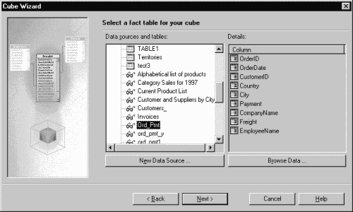
dialog boxes appearing. In the first dialog box, we
need to select the data source for our cube. For doing this, it is necessary to
select OLE DB Provider for MS SQL Server, and then choose a fact table
containing data for summaries. Let it be our Ord_pmt view,
created earlier.
Then, we will be asked what
numeric values should be used as cube measures (as we have said before,
measures are the source data for creating summaries). In the Ord_pmt
view, there are three numeric fields - the OrderID, Freight and Payment
fields. Let's select both Freight and Payment fields as cube
measures. In the next dialog, we need
to define dimensions of the cube. For doing this, we can press the New
Dimension button, and the Dimension Wizard occurs. For creating all
necessary dimensions, we need to run the Dimension Wizard four times. Let the first dimension is
the OrderDate. In the first dialog box of the Dimension Wizard, we will
select the same Ord_pmt view as a dimension source. In a general case,
the source of dimension can be any other table of view, which is in the lookup
relation with the fact table or view. In the second dialog, we need to select
the type of dimension. Let it be a time dimension. In the third dialog, it is
necessary to choose a type of date/time hierarchy. As our data contains no
time, we will select 'Year, Quarter, Month, Day' type of hierarchy. We
also can point, where a year starts. It is very useful, when, for example, the
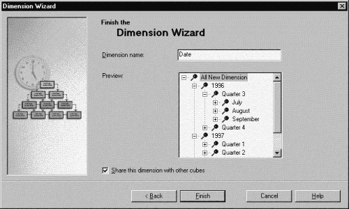
fiscal year is not the same as the calendar year. At last, we can name the
created dimension as Date, and browse all hierarchy levels of this
dimension:
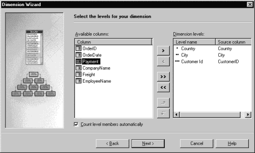
The next step is to create
another dimension. Let it be the Country/City/CustomerId dimension. In
fact, this dimension contains three levels of "geographical"
hierarchy, because in this example any customer resides in the particular city
and country. Therefore, we should select the Country, City and CustomerId
fields to be the levels of the hierarchy of this dimension:
The third dimension is very
simple. It contains only the CompanyName field. At last, the fourth dimension
also contains only one EmployeeName field. Finishing creating all four
dimensions, we need to save the cube. Then, we will be asked, what type of data
storage must be created: MOLAP (Multidimensional OLAP; it means that all
data, both source and aggregates, is stored in a multidimensional database, and
this way is recommended for use with analytical applications), ROLAP
(Relational OLAP; all data are stored in a relational database, and this way is
recommended to use in applications responsible both for data modification and
analysis), or HOLAP (Hybrid OLAP; aggregate data is stored in a
multidimensional database, and source data is stored in a relational database).
We will select the MOLAP data storage. After that, we can also set some storage
options to provide a necessary balance of the storage size and the performance
of user query executing. Then, we are able to
process the cube, i.e. to calculate aggregate data. At any time, you can edit
the created cube. It is also possible to create it in editor without using
wizards. In addition, we could create it directly from tables instead of
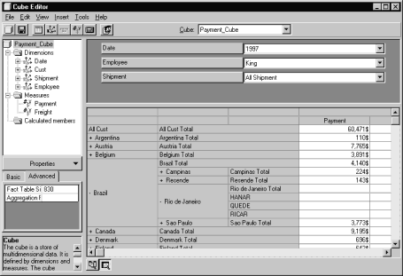
creating views. After processing the cube,
we can view its data. It can be done by selecting the View/Data option
from the Cube Editor menu. In the Cube Editor, we can drag-and-drop
dimensions, show and hide them, expand and collapse hierarchy levels, move
dimensions from columns to rows, filter cube data by selecting possible values.
Thus, we have prepared all
necessary server data. We have created an OLAP cube based on previously created
view. It has four dimensions:
And, in addition, this cube
has also two measures:
Thus, we have created the
cube with aggregate data. Now we need to create applications to access its
data. But, before querying cubes, a user needs to know, what cubes are
contained in multidimensional database, what are their dimensions, hierarchies,
levels, and their members. In other words, a user needs to know, what query
parameters could be used. In the next section, we will show how to do it using the
OpenSchema method of the TADOConnection component. Retrieving
Cube Metadata in Delphi Applications
How to obtain information
about cubes, their dimensions, hierarchies, levels, and their members in Delphi
applications? Let's recall, that we have already studied how to do it with
relational databases. The OLAP cubes created with
Microsoft SQL Server 7.0 OLAP Services can belong to multidimensional database
that must not be of relational type. But, in spite of this, they are accessible
via Microsoft OLE DB Provider for OLAP Services. So, to retrieve the
cube metadata, we are able to use the OpenSchema method of the ADO
Connection object that is accessible through the Delphi TADOConnection component.
Looking carefully to the
list of possible values of TSChemaInfo parameter, we can find some of
them concerning to cubes. They are siCubes, siDimensions, siHierarchies,
siLevels, siMeasures, siProperties, siMembers values. Using them as the
first parameter in the OpenSchema method, we can retrieve information on cubes,
dimensions, their hierarchies, levels, measures, members in the particular
multidimensional database. Let's create an example of
using this method to retrieve cube metadata. For doing this, we need to create
a new Delphi project, and place the TComboBox, TButton, TDBGrid,
TDBNavigator, TADOConnection, TADODataSet, TDataSource components on a
form. Then, let's set the DataSource value of the DBNavigator1
and DBGrid1 components to DataSource1, the DataSet
property of the DataSource1 component to ADODataSet1, and fill
the Items value of the TComboBox component with the following
strings:
Then, let's set up the Connection
property of the ADOConnection1 component. We need to select the Microsoft
OLE DB Provider for OLAP Services as a provider name, input or select the
computer name with multidimensional database as a data source name, insert the
user name and password, and then select the multidimensional database name
which metadata we want to retrieve. The next step is to create
the OnClick event handler for the Button1 component:
And, at last, let's
initialize the ItemIndex property of the ComboBox1 component:
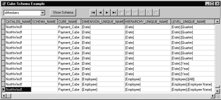
Now we can compile and run
this application. The example of its output is shown below:
If we need to filter the
retrieved metadata, we could define the criteria what metadata to show. This
criteria must be the second parameter of the OpenSchema method, and it
contains an array of values for filtered columns of the resulting dataset. For
example, if we want to show only the members of the Employee dimension
of the Payment_Cube cube of the NorthWind1 multidimensional
database, the following code could do it:
Now we know how to retrieve
the cube metadata into the client Delphi application. Now we can find, what
cubes are available, and what are their dimensions, hierarchies, levels and
members. So, we have enough information to create queries to the cube. However, in most of the cases,
we are interested both in cube metadata and in cube data. In a general case, it
is necessary to query the cube to obtain its slices, and then show them in a
client application, with these queries being based on the knowledge about the
cube metadata. So, now it is time to
create queries that can be used in a client Delphi applications. For querying
cubes, the Multidimensional Expressions (MDX) are used. Multidimensional
Expressions are an SQL language extensions used for querying cubes accessible
through OLE DB Provider for OLAP Services. We will provide a brief
description of these SQL language extensions in the next section. Using
Multidimensional Expressions (MDX)
OLE DB for OLAP is a set of
COM interfaces designed to extend OLE DB for efficient access to
multidimensional data. For expressing queries to multidimensional data stored
in SQL Server OLAP cubes, OLE DB for OLAP employs multidimensional expressions
(MDX), which are extensions of SQL. OLAP Services supports MDX functions as a
full language implementation for creating and querying cube data. We will provide a brief
description of the Multidimensional Expressions. But, before this, we need to
create a test application to execute MDX queries. The MDX Test Application
Before studying the details
of MDX, we need a Delphi application that will allow us to enter various MDX
statements and immediately see the results of their execution. For doing this,
we will create a simple application containing the TDBGrid , TMemo,
TADOCOnnection, TADOQuery, TDataSource, TButton component. Then, we need to
set change the ConnectionString property of the TADOConnection
component. We will to select Microsoft OLE DB Provider for OLAP Services,
then select the server name and database name, as usual, and, in this case, the
name of initial catalog to use should be NorthWind1 (e.g. the name of
our database, which contains the previously created cube). Then, let's create
the OnClick event handler of the Button1 component:
Now this application is
ready for use. A Brief Overview of
Multidimensional Expressions (MDX)
Now we can begin our short
tour on MDX queries. To create them, we need to take into account the
information about the cube metadata obtained through the OpenSchema
method of the ADO Connection object, and to test them, we can run a test
application created before. The MDX syntax
The simplest form of MDX
query is: SELECT axis_specification ON COLUMNS,axis_specification ON ROWS FROM cube_nameWHERE slicer_specification
The axis specification can
be thought of as the member selection for the axis. A member is an item in a
dimension or measure. The slice specification on
the WHERE clause is optional. If it is not specified, the returned
measure will be the default for the cube. Unless you actually query the
measures dimension, you should always use a slice specification. The MEMBERS function
The simplest form of an
axis specification or member selection involves taking the MEMBERS of
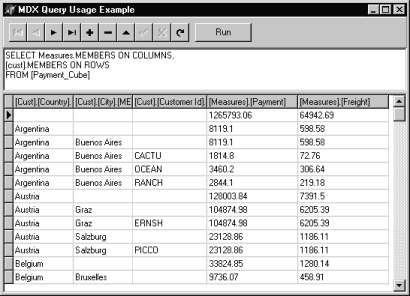
the required dimension, including those of the special measures dimension: SELECT Measures.MEMBERS ON COLUMNS,[cust].MEMBERS ON ROWSFROM [Payment_Cube]
This expression satisfies
the requirement to query the recorded measures for each customer along with a
summary at every defined summary level. Alternatively, it displays the measures
for the cust hierarchy. In running this expression, we can also observe an
unnamed row member in the first row. It contains summaries for measures for all
customers. Such "All " member is generated by default. The result of such query is
shown in the figure below:
In addition to taking the
MEMBERS of a dimension, a single member of a dimension can be selected. SELECT Measures.MEMBERS ON COLUMNS,{[cust].[Country].[France],[cust].[Country].[Germany]} ON ROWS FROM [Payment_Cube]
This expression queries the
measures summarized for the orders in of France and Germany. The CHILDREN function
To actually query the
measures for the members making up both these countries, it is necessary to
query the CHILDREN of the required members: SELECT Measures.MEMBERS ON COLUMNS,{[cust].[Country].[France].CHILDREN,[cust].[Country].[Germany].CHILDREN} ON ROWSFROM [Payment_Cube]
What is the difference
between CHILDREN and MEMBERS? The MEMBERS function returns the members for the
specified dimension or dimension level, and the CHILDREN function returns the
child members for a particular member within the dimension. For example, in the
query above, [cust].[Country].[France].CHILDREN are cities in France,
but [cust].[City].MEMBRES are all cities where customers resides. The DESCENDANTS function
Both CHILDREN and MEMBERS
functions can be used in formulating expressions, but they do not allow to drill
down to a lower level within the hierarchy. This can be done by the DESCENDANTS
function. This function allows go to the next level in depth. Its syntax is the
following: DESCENDANTS(member, level [, flags])
If the flags parameter is
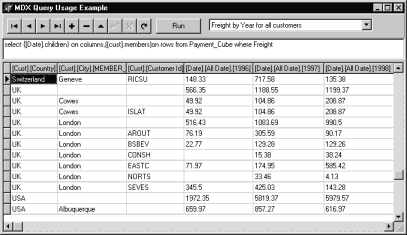
omitted, the members at the specified level will be included, for example: SELECT {[Measures].[Payment]} ON COLUMNS,(DESCENDANTS([cust].UK, [City])) ON ROWSFROM [Payment_Cube]
In this case, in the rows
axis, we will receive the members of the City level of the cust
hierarchy for the UK member of the Country level, as it is shown
in the figure below: The same result will be
received, if we use the SELF flag value. If we use the AFTER flag,
we will drill down to the depth in the next level of the hierarchy in the rows
axis: SELECT {[Measures].[Payment]} ON COLUMNS,(DESCENDANTS([cust].UK, [City], AFTER) ) ON ROWSFROM [Payment_Cube]
In this case, we will
receive several rows for all customers in the United Kingdom. If we use the BEFORE
flag, we will receive the higher level of a hierarchy on the axis. In this
case, we will receive only one row for the UK member. At last, if we use the BEFORE_AND_AFTER
flag value, we will receive the several rows for the next level of a hierarchy,
and the row for the highest level: SELECT {[Measures].[Payment]} ON COLUMNS,(DESCENDANTS([cust].UK, [City], BEFORE_AND_AFTER) ) ON ROWSFROM [Payment_Cube]
The Slicer Specifications
To define what data must be
output, we need to define a slicer specification. Let's look at the following
example: SELECT {[Date].CHILDREN} ON COLUMNS,([cust].MEMBERS)ON ROWSFROM [Payment_Cube]WHERE Payment In this case, we obtain
two-dimensional set of summaries of payments for any customer and any year. The next example shows
shipment expenses in Quarter 2 of 1998: SELECT {[Shipment].children} ON COLUMNS,([cust].members)ON ROWSFROM Payment_CubeWHERE ([Date].[Year].[1998].[Quarter 2]) In this example, we have
defined how to select a specific data range in the slicer specification. Note. Slicing does not affect selection
of the axis members. It affects only the values that go into them. This is not
the same as filtering, because filtering reduces the number of axis members. This was a little intro to
MDX queries. In fact, they can also use calculated expressions
(including conditional expressions), create slices for comparing parallel
periods (e.g. January 1997 and January 1998), provide filtering and sorting
data, use calculated members (dimension members, whose value is calculated at
run-time), and provide many other useful facilities. Now we can modify our test application by adding a predefined queries. For
doing this, let's add the TComboBox component and fill it with the
following strings:
At last, let's create an OnChange event handler for the ComboBox1 component.
Now we can compile and run the application. After selecting the type of
query, the appropriate result set is shown in a grid.
Thus, in this section we have looked at the way how to create a simple
Delphi client for SQL Server OLAP Cube using an appropriate OLE DB Provider and
ADO components. Using ADO MD Extensions
The Microsoft Data Access Components (MDAC) contain more than core
ADO objects. Version 2.1 comes with the some extensions, and, among them, there
is ADO extension to work with multidimensional data that first appeared in the
ADO 2.0. In this section, we will take a look at ADO MD Extensions, their object
model and features, and give you some examples of how to use them. Note that
all this functionality comes with a single installation file - MDAC_TYP.EXE
that ships with Delphi 5 Enterprise and for purchase with Delphi 5 Professional,
and is also available in the Microsoft web site for download. ADO MD
Extensions, along with ADO Extensions for DDL and Security (ADOX), are
available without requiring some extra installation. ADO MD Objects
As all other interfaces in Microsoft Data Access Components, ADO MD consists
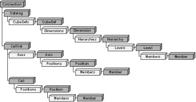
of a set of objects. The following diagram shows what objects comes with ADO
MD, and how they are related to each other.
As we can see from the diagram above, the main objects of ADO MD are Catalog
and CellSet.
Accessing ADO MD from Delphi
Since ADO MD support in Delphi 5 was not implemented at the components
level. We need to use the type library to access ADO MD objects. This type
library resides in msadomd.dll file. To do so, choose the Project |
Import Type Library command from the main menu and in the Import Type
Library dialog box select Microsoft Microsoft ActiveX Data Objects
(Multi-dimensional) 1.0 Library. If you have already imported ADOX type library, you need to avoid conflicts
with already declared Delphi TCatalog class. In this case, just rename TCatalog
into TADOMDCatalog. It is also better to uncheck the Generate
Component Wrapper checkbox because we need only to create a *.pas
file to access ADO MD objects. Then press the Create Unit button. We will end up with the ADOMD_TLB.PAS file, that is Pascal language
conversion of the contents of the ADOMD type library. In the most of examples,
we will assume that the ADOMD_TLB.PAS file is included in the Uses clause. Note. Since we will use some COM functions, as well as
several routines, implemented in the ADO MD, we will need to include the COMOBJ
and ADODB units into the Uses clause. ADOMD Usage Examples
Now we will create several examples to illustrate how to use ADO MD objects.
We will show how to use the Catalog object to retrieve cube metadata, and how to
them will show you how to use the CellSet object and its collections. Using the Catalog Object and its Collections
To show how to use the Catalog object and its collections, we will
create three examples. The first one will show you how to get cube names and
properties. The second one will show you how to obtain dimension properties. At
last, the third one will show how to obtain the names of levels and members. Getting Cube Names and Properties
In our first example, we will get a list of cubes within a selected catalog.
For doing this, we will iterate the CubeDefs collection of the Catalog
object, extract the CubeDef object, and get its properties. We will show
cubes available in a tree structure, so we will use a TTreeView
component from the Win32 page of the Component Palette. Place it into a form
along with a TButton component. First, we need to create an instance of a Catalog object. Here is a
code to do this:
This line of code creates a COM object based on the object name. We store the Catalog1 variable and the CubeDef1 variable in
the global declaration section. Later we will add some more such variables
there.
Next, we need a name of the data source where the tables are stored. We use
the standard Delphi function PromptDataSource from the ADODB unit
to get one and save the value it returns in the global variable DS:
The real stuff is implemented inside the CubeList procedure, which
procedure can be split up into two parts, the TreeView1 initialization
part and the cubes iteration part. In the first part, we create a root node and
a child node for cubes. Next, we connect our selected data source to the Catalog
object:
After that, the data source will be opened, and we can traverse through the
cubes within it. First, we check that we have cubes. This is not necessary,
since any actual storage should have at least one cube. We do this just to show
you how to use Count property of the CubeDefs collection.
Now we enter the loop, where at each step we extract one CubeDef
object at a time and show it in the TreeView1 component. Here is the
code we use for this:
Then, we need to get the CubeDef object properties by iterating its Properties
collection and show them in the TreeView1 component. First, we check that we have at least one property in this collection.
Second, we enter the loop, where at each step we extract one Property
object at a time and show its name and value in the TreeView1 component.
For doing this, we use the Name and the Value properties of the Property
object. Here is the code we use for this:
Thus, the full source code of the CubeList procedure will look like
that:
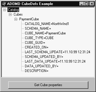
After saving and compiling this project, we can obtain the following output
in the TreeView1 component:
Getting Dimension Properties
In our second example, we will get a list of dimensions and their properties
within a selected catalog. For this, we will iterate the Dimensions collection
of the CubeDef object, extract the Dimension object and get its
properties. It is a modified version of the previous example, so it also uses a
TTreeView component. As in the previous case, we also need to create an instance of a Catalog
object, and obtain the data source name using the PromptDataSource
function. Let's also add to the global declaration section the next line:
As the real stuff is implemented inside the CubeList procedure, we
need to modify it a little:
This procedure looks like the same one from the previous example. But there
are some differences. As in the previous case, we need to connect the Catalog
object to our selected data source, and then traverse through the cubes
within it. Also, as in the previous case, we enter the loop, where at each step
we extract one CubeDef object at a time and show it in the TreeView1
component. But then, we need to obtain dimensions and their properties for each cube.
To do this, we call the ShowDimProp procedure. Its code looks like that:
Let's look at this procedure in more details. First, we need to get the Dimension
collection of the CubeDef1 object, check whether it contains at least
one dimension, iterate it, obtain the Dimension object from it and add its name
to the TreeView1 component:
First, as in the previous example, we check that we have at least one
property in this collection. Second, we enter the loop, where at each step we
extract one Property object at a time and show its name and value in the
TreeView1 component. Here is the code we use for this:
After saving and compiling this project, we can obtain the next output in the TreeView1 component:
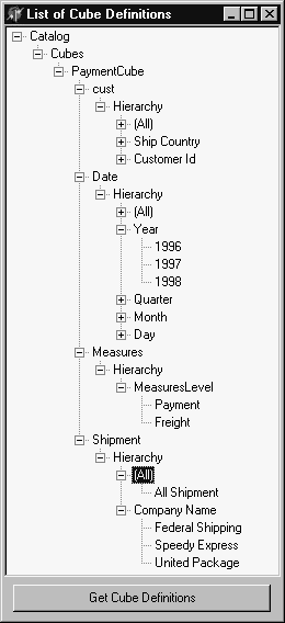
Getting Names of Hierarchies, Levels and Members
In our third example, we will get a list of all objects inside the selected
catalog, i.e. cubes, dimensions, their hierarchies, levels and members. For
this, we will iterate all collections of all objects within hierarchy of the Catalog
collections. It is also a modified version of the previous example, so it
also uses a TTreeView component. As in the previous example, we also need to create an instance of a Catalog
object, and obtain the data source name using the PromptDataSource function.
Let's also add the following lines to the global declaration section:
As the real stuff is implemented inside the CubeList procedure, we
need to modify it a little again:
This procedure is almost the same as one from the previous example. But
there are some differences. As in the previous case, we need to connect the Catalog
object to our selected data source, and then traverse through the cubes within
it. Also, as in the previous case, we enter the loop, where at each step we
extract one CubeDef object at a time and show it in the TreeView1
component. Then, we also need to obtain dimensions for each cube. To do this, we call
the DimList procedure: Its code looks like that:
Instead of iterating the Property collection of the Dimension1
object, we need to iterate its Hierarchies collection. So, we need to check
that we have at least one hierarchy in this collection. To obtain a list of hierarchies of the dimension, we call the HierarchyList
procedure. It looks like that:
Here we enter the loop, where at each step we extract one Hierarchy object
at a time and show it in the TreeView1 component. Then, we need to know
is there any level in this hierarchy. We need to comment the following line:
It is used for the case, when the Name property of the Hierarchy object
returns an empty string. Our cube just contains unnamed Hierarchy objects, one
for each dimension. At the next step, if there are levels in this collection, we need to iterate
the Levels collection of the Hierarchy object. The LevelList
procedure is designed for this:
At last, we need to check that we have at least one member in the Members
collection of the Level object, and, in the case we have one, to iterate
the Members collection of the Level object. The MemberList procedure
is designed for this:
Here, we enter the loop, where at each step we extract one Member object
at a time and show it in the TreeView1 component. After saving and compiling this project, we can obtain the following output
in the TreeView1 component:
Using CellSet Objects
To show how to use the CellSet object and its collections, we will
create two examples. The first one will show you how to retrieve the members of positions along Axis
objects of the Axes collection of the CellSet object, how to
retrieve the Cells values using the Item method, and place all
obtained values into a grid. The second one will show you how to retrieve the
same data to the client dataset. Retrieving Cells to a Grid
In this example we will create a CellSet object and put the values of
its cells into a grid. Also, we will draw a chart with the CellSet
content. For doing this, we will iterate through all Cell values
available by using the Item method of the CellSet object. Let's start a new project and place the TStringGrid component, TButton
component, TChart component on a form. Also, let's place on the form
the TComboBox component (we will fill it with names of some predefined
MDX queries), and TMemo component (it will contain the text of an MDX
query, which can be edited by the user). You can arrange these components as
you like, set the necessary Align properties, use toolbars, splitters,
etc. As opposite to the examples shown earlier, let's use Automation with
Variants instead of using interfaces, because this results in more simple code.
First, let's prepare a set of pre-defined MDX queries, and place their names
to the ComboBox1.Items property, for example:
The MDX query text itself will be placed to the Lines property of the Memo1
component. For doing this, we need to create the OnChange event handler
for the ComboBox1 component:
This event handler places the appropriate text of an MDX query, when the
user selects an item from the ComboBox1. In addition, the user can just
edit the Memo1 content at run-time to retrieve CellSets that
results from the custom MDX queries. Second, we need to provide a Variant variable to work with when creating an
instance of the CellSet object. We store this variable in the global
declaration section:
Next, we need a name of the data source where the cubes are stored. We use
the standard Delphi function PromptDataSource again to get one, and save
the value it returns in the global variable DS:
As you can see, we put this code in the Button1 event handler - when
the user presses the button, he faces the data source selection dialog. When
one is selected, i.e. DS variable is not empty string, we call the CellGrid
procedures passing the data source name as an argument, and then call the CellChart
procedure to draw a chart using the StringGrid1 data.
First, in this procedure we must create an instance of the CellSet object:
Second, we need to open this CellSet using the data source obtained
from the PromptDataSource function, and the text of an MDX query taken from the
Memo1 component.
Third, we need to find out, how many columns and rows the StringGrid1 component
must contain. For doing this, we need to use the Count properties of the
Positions collections of the Axis objects, which belong to the Axes
collection of the CellSet object:
As we have discussed earlier, usually there are two Axis object in
the Axes collection - the first one for columns (Axes[0]), the second
one for rows (Axes[1]). As we need to have an additional row for column
names and an additional column for row names, we add one to the value of the Count
properties for both axes. Forth, we need to fill the first column of the StringGrid1 component
with the row names. To do this, we need to iterate all Position objects
of the Positions collection of the appropriate Axis object (in
this case, it is the CellSet1.Axes[0] object) . We can get the row name
from the Caption property of the primary item of the Members collection
of such Position object:
Fifth, let's also fill the first row of the StringGrid1 with the
column names. To do this, we need to iterate all Position objects of the
Positions collection of the appropriate Axis object (now it is
the CellSet1.Axes[0] object):
Sixth, let's fill the rest of the StringGrid1 components by the CellSet
content. For doing this, we need to obtain the necessary values by using
the Value property of Cell objects that are returned by the Item
method of the CellSet object:
We put zero to all empty cells of the StringGrid1. This component
itself does not require filling such cells by data. But later we will create a
chart with this data, so it is necessary to have a valid numbers in these
cells. At last, we need to close the CellSet object and de-assign the
Variant variable:
To provide a good user interface for our application, let's create a chart
with the StringGrid1 data. The CellChart procedure is designed to
do this:
First, we need to clear the series list of the Chart1 component.
Second, we need to iterate all columns to create appropriate series of the
chart:
At last, we need to add points to all specific series:
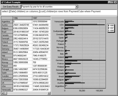
The result of retrieving cells to a string grid and a chart is shown below.
Retrieving Cells to a Client Dataset
The next example will show you how to retrieve the Cell object values
data to the client dataset. It can be useful if you need to use facilities of
future processing this data in a client application, e.g. sorting, filtering,
generating reports or HTML contents. In this example we will create a CellSet object and put the values in
its cells into the TClientDataSet component. As in the previous example,
we will draw a chart with the CellSet content. For doing this, we will
also iterate through all Cell values available by using the Item method
of the CellSet object. Let's start a new project and place the TClientDataSet component, the
TDBGrid component, the TDBNavigator component, the TButton component,
the TChart component on a form. Also, let's place on the form the
TComboBox component (as in the previous example, we will fill it with names
of predefined MDX queries), and the TMemo component (as in the previous
example, it will contain the text of MDX query, which can be edited by the
user). You can arrange these components, set the necessary Align properties,
use toolbars, splitters, etc. As in the previous example, we will use Automation with Variants instead of
using interfaces. First, let's prepare a set of pre-defined MDX queries. Let they be the same
as in the previous example. As in the previous example, the MDX query text will
be placed to the Lines property of the Memo1 component. So we
will place the MDX query names into the Items property of the ComboBox1 component,
and create the same the OnChange event handler for the ComboBox1 component
(see the description of the previous example for details). Second, we need to provide a Variant variable to work with when creating an
instance of the CellSet object. We store it variable in the global
declaration section:
Next, we also need a name of the data source where the cubes are stored. We
use the standard Delphi function PromptDataSource to get one, and save the
value it returns in the global variable DS:
As in the previous case, we put this code in the Button1 on click
event handler. When the data source is selected, we call the CDSFill procedures
passing the data source name as an argument, and then call the CDSChart procedure
to draw a chart using the CellSet data. The real stuff is implemented inside the CDSFill procedure, source
code of which looks like that:
First, in this procedure we must create an instance of the CellSet object
and open it:
Second, we need to create the first field of the client dataset. It will
contain the row names, so it will be of a string type.
Third, we need to create fields to store the CellSet data. These
fields must be of a Float type.
We need to comment this code. The reason of using the Ordinal
property in the field name is that field names must be unique in the dataset.
But we can have the same Caption properties for different positions. For
example, look at the next MDX query: select {[Date].[1997].[Quarter 1], [Date].[1998].[Quarter 1]}on columns, ([cust].children)on rows from PaymentCube where Payment The result of this query will contain two columns with the same name Quarter
1. But in this case we cannot use these names as field names. As for Ordinal
value, it is unique, so we can add it to the field name. You can, of course, provide any other way to obtain unique names of your
fields. For example, you can use the UniqueName property of the
appropriate member instead of using Caption property:
Fourth, we need to create the client dataset and open it.
Now we need to iterate the CellSet rows and add each of them to the
client dataset. First, we need to append a record to the client dataset:
Second, we need to insert data into the first field of the created record.
It will be the name of the Cellset row. So, we need to use the Caption
property of the primary member of the current Position object, that is
an item of the Positions collection of the appropriate axis. In this
case, it is the CellSet1.Axes[1] object:
Third, we need to fill the rest fields of the record. The values to be
inserted are the Value properties of the Cell objects that are
results of executing the Item method of the CellSet object.
At last, we need to close the CellSet object and de-assign the
Variant variable:
To provide a good user interface for our application, let's create a chart
with the ClientDataSet1 data. The CDSChart procedure is designed
to do this:
First, we need to clear the series list of the Chart1 component.
Second, we need to iterate all columns to create appropriate series of the
chart:
At last, we need to add points to all specific series:
The result of retrieving cells to the client dataset and an appropriate
chart is shown below.
Pros and Cons of Delphi Server-side OLAP applications
Using server-side OLAP looks more advantageous that using client-side one. The important advantage of such way of creating OLAP applications is that in
this case you can provide on-line analytical processing possibilities without
bringing a lot of data to the client application. In this case, all necessary
calculations are provided by the database server, and the end user obtains only
slices from it. In addition, modern OLAP extensions, such as considered above,
can provide enough possibilities for choosing optimal balance between
performance of server calculations and the server storage size. And, at last,
querying cubes from client applications is also available. It is not very
difficult to create a client application, which generates necessary queries. If we discuss the particular Delphi implementation of server-side OLAP with
ADO data sources, we can see that it is not very difficult to create
server-side OLAP applications with the user interface similar to the interface
of applications with the Decision Cube components. However, this way of creating OLAP applications also have a little
disadvantage. We have seen, that we can easily use OLE DB provider for SQL
Server OLAP Extensions. But if we use OLAP extensions of other vendor, we have
not any guarantee, that an appropriate OLE DB provider is already available.
So, in a general case, we need use Microsoft SQL Server for providing
server-side OLAP possibilities, even if we want to store data in another
database server (we have mentioned above, that the data sources for creating
OLAP cubes can differ from MS SQL Server). But we hope that this problem seems
to be solved just in the nearest future. It should be mentioned, however, that other OLAP vendors sometimes provide
some client objects to add possibility of using their server-side OLAP, such as
ActiveX controls (and, of course, SQL Server OLAP Extensions does too). But
this is out of the scope of this book. Conclusion
In this article, we have provided an introduction to On-Line Analytical
Processing (OLAP). Now we know that:
Also, we have discussed two ways of implementing OLAP in Delphi application
- the client-side OLAP and the server-side one. Now we know that:
We have also discussed one of particular implementation of the Delphi
server-side OLAP based on using the OLAP extensions implemented in Microsoft
SQL Server 7.0 along with Delphi ADO components. We have described how to
create multidimensional cube, and how to process it, and how to access the cube
metadata and data from Delphi. Now we know that:
Also, we have discussed using
server-side OLAP Delphi applications using ADO MD objects. Now we know
that:
We have also discussed
advantages and disadvantages of using server-side OLAP for creating OLAP
applications. We see that this way is free from such disadvantage as bringing a
lot of data to the client. It can be used with large data sources, because in
this case all summaries are calculated by the database server. Modern OLAP
server-side software, such as OLAP Extension for MS SQL Server 7.0, provides a
lot of possibilities to bring summaries to client applications, including OLE
DB provider for OLAP Extensions and ADO MD extensions, and this make it
possible to create Delphi clients for such OLAP servers. | |||||||||||||||||||||||||||||||||||||||||||||||||||||||||||||||||||||||||||||||||||||||||||||||||||||||||||||||||||||||||||||||||||||||||||||||||||||||||||||||||||||||||||||||||||||||||||||||||||||||||||||||||||||||||||||||||||||||||||||||||||||||||||||||||||||||||||
|
За содержание страницы отвечает Гончарова М.Н. © Кафедра СПиКБ, 2002-2017 |
||||||||||||||||||||||||||||||||||||||||||||||||||||||||||||||||||||||||||||||||||||||||||||||||||||||||||||||||||||||||||||||||||||||||||||||||||||||||||||||||||||||||||||||||||||||||||||||||||||||||||||||||||||||||||||||||||||||||||||||||||||||||||||||||||||||||||||


 At
last, we need to get the Dimension1 object properties by iterating its Properties
collection and show them in the TreeView1 component.
  Here we
enter the loop, where at each step we extract one Level object at a time
and show it in the TreeView1 component.